Predictor based on adaptive simulated annealing¶

See Wikipedia and also simulated annealing for basics.

The adaptive simulated annealing part of adviser’s resolution algorithm takes either a top rated state for expansion or, based on probability, picks some another state from the beam. This state is expanded by picking one dependency from unresolved dependency listing and obtaining its direct dependencies making the dependency resolved and direct dependencies becoming part of unresolved dependency listing. The probability of picking a neighbour state (and not the highest rated stack) from beam is computed based on, besides other parameters, the temperature function which respects number of iterations and number of final states produced so far (thus “adaptive” simulated annealing).

See adaptive simulated annealing implementation.

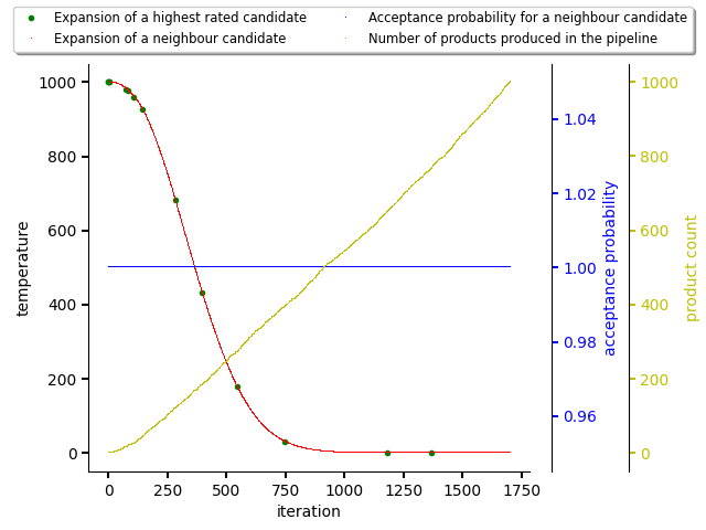
An example of an adaptive simulated annealing run that produced 1000 Python stacks (final states) with no observations on scored packages seen on the following figure. As the database for scoring states is empty (Python stacks were just resolved without any guidance), the probability of picking a random state from the beam is high (the algorithm is looking for a state which would be better than a score of 0.0 in comparision to a neighbour candidate with a score of 0.0). This acceptance probability is kept even as the temperature drops.

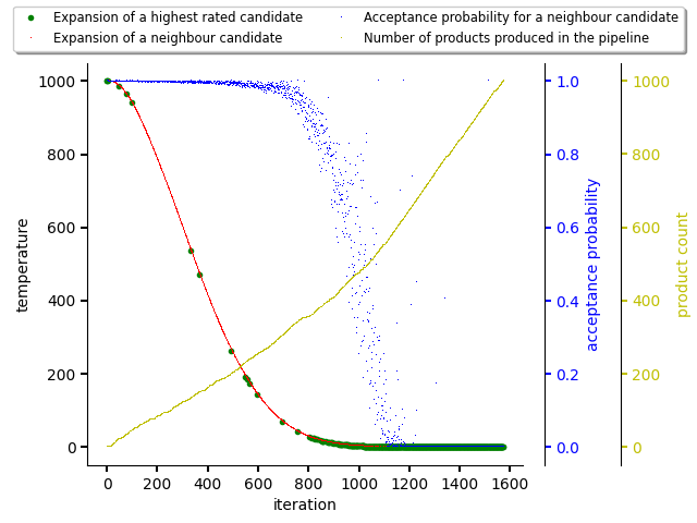
On the figure below, there was created a random dataset for scoring packages in the resolution process for demonstration purposes. As can be seen, the acceptance probability for picking a neighbour state for expansion is decreasing with number of final states produced and with decreasing temperature during iterations. This caused picking the highest rated states for expansion and producing final states out of them (fully resolved Python software stacks). Once temperature drops to 0.0, only highest rated software stack is picked for resolution as acceptance probability for the neighbour state dropped to 0.0 as well.

Temperature coefficient¶

Predictor based on adaptive simulated annealing (and all the derived ones), accepts a parameter called temperature_coefficient. This parameter is used to specify how steep the temperature decrease should be. For reinforcement learning based predictors (see Predictor based on Monte Carlo Tree Search (MCTS) and Predictor based on Temporal Difference learning (TD-learning)) this parameter balances exploration and exploitation phases. A usual values for this parameter are 0.9<=temperature_coefficient<1.0.

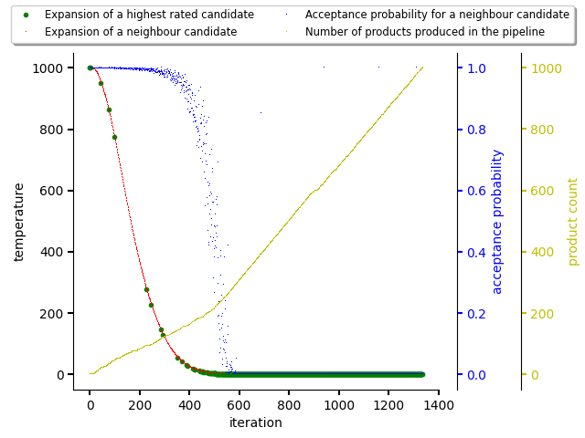
The figure below shows a simulated annealing run when temperature_coefficient is set to 0.9.

In comparision to figure above, the figure below shows another simulated annealing run when temperature_coefficient is set to 0.98.

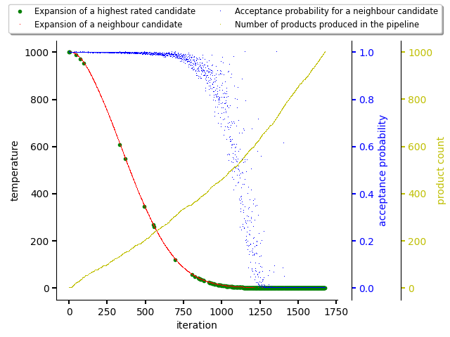
Even though in both cases there were used same input data and same seed for random generator, results differ as steps taken by resolver differ across iterations.

It’s worth to adjust this parameter in a deployment based on time allocated for adviser runs. The right value should make sure adviser is able to sample the state space and perform exploitation of highest states found considering CPU time allocated in the cluster pre a resolution request. See also Configuring and setting up resolver in a cluster section.