Predictor based on Monte Carlo Tree Search (MCTS)
Note
Check high level predictor docs for predictor basics.
This method is also many times referred as “Monte Carlo learning”.
See Wikipedia for a brief intro to MCTS.
The core idea lies in creating “trajectories” into dependency graph and learn policy for which the software stacks should be resolved based on the reward obtained.

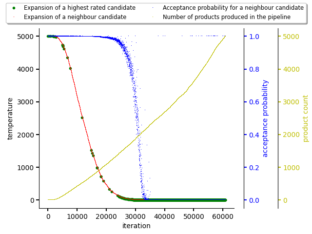
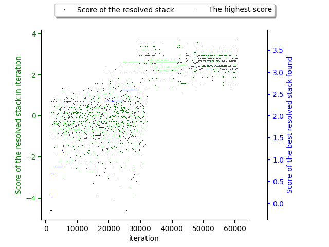
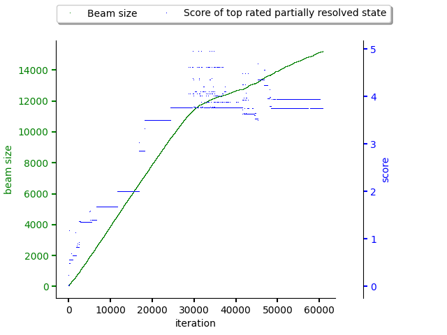
The figures below show a resolution that is guided using an MCTS predictor.
The very first figure shows exploration and exploitation phases balancing using annealing schedule. As can be seen, the exploitation phase finishes roughly in iteration 30000 when the acceptance probability for expanding a neighbour candidate drops to 0 and only the highest rated candidates are expanded (exploitation).

Note
The exploration and exploitation phase is balanced using an annealing
schedule. The balance factor can be parametrized using
temperature_coefficient parameter that can be supplied to the predictor.
see reinforcement learning intro section for more info.
The second figure shows how software stacks produced by resolver increased they score during the exploitation phase until circa 30000 iteration. This corresponds to start of the exploitation phase. No better software stack was resolved since then.

The last figure shows size of the beam keeping unresolved (partially resolved) states. The max score of partially resolved states increase until iteration 30000 (exploration phase) and then the max score for partially resolved states relatively stabilizes. It’s also good to spot how the beam size behaves. Once the exploration phase finishes, beam size does not increase that drastically.

It’s also worth to point out the dataset used when creating plots was made out of sparse scores.
See this notebook that shows the resolution process using MCTS predictor.